Introduction in the gradient descent

A bit of theory:

Suppose we just need to find a minimum of the one-dimensional function.

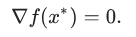
As early as the 17th century Pierre de Fermat was invented a criterion that allowed solving simple optimization problems, namely, if x* is a minimum point of f*, then:

This criterion is based on a linear approximation

The closer x to x*, the more accurate this approximation

In the multidimensional case, similarly:

Our criterion can be written as:

It should be noted that our function F must be convex.

The value  is the gradient of the function f at a point x*. Also, the equality of the gradient to zero means the equality of all partial derivatives to zero, so in the multidimensional case, we can get this criterion simply by consistently applying the one-dimensional criterion for each variable separately.

What happens if the gradient is not zero?

If gradient  , then the gradient indicates the direction of the greatest local increase of the function . From this is based the method gradient descent.

Graphically Gradient descent can be portrayed so:

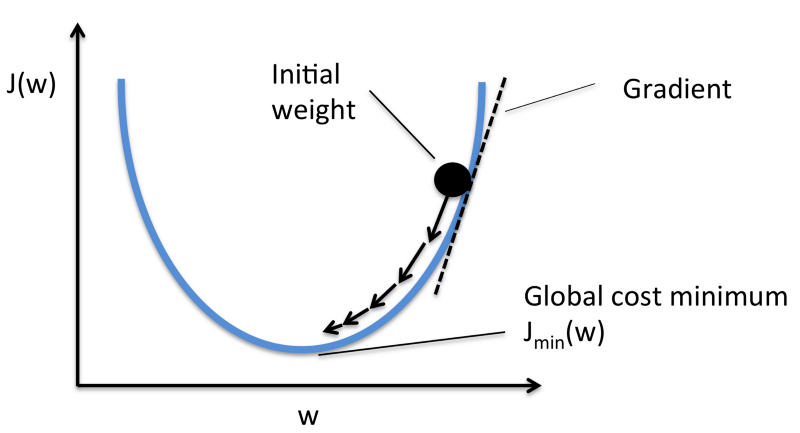
So, suppose we have a simple function J = w2. We know that the minimum of the function is at w = 0, but suppose we do not know it. Our weight coefficient is set randomly. Suppose w = 20.

The derivative dJ/dw is 2w. Set the learning rate to 0.1. In the first approximation, we have:

w – 0,1*2w = 20 – 0,1*40 = 16

w = 16. In the second approximation:

w – 0,1*2w = 16 – 0,1*2*16 = 12,8

w = 12.8. In the third approximation:

w – 0,1*2w = 12,8 – 0,1*2*12,8 = 10,24

Essentially a gradient descent can be described by the formula:

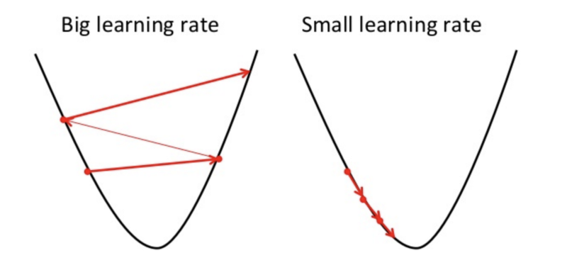
The value α_k is called the step size (in machine learning, the learning rate). A few words about the choice α_k: if α_k is very small, then the sequence is slow, which makes the algorithm not very effective; if α_k is very large, then the linear approximation becomes bad, and maybe even incorrect.